The Main Problem-Solving Method
The Importance of How You First Approach a Problem
Most problems (and sub-problems) are very easy to solve and should usually be solved in a couple of seconds or less. Such a claim may seem outrageous because usually people don’t consciously consider such simple problems as problems. An important rule that applies to many situations is the Pareto rule (which is based on the Pareto distribution in statistics). This rule is usually stated as: 80% of your success comes from 20% of your effort, and the other 20% of your success comes from the remaining 80% of your effort. Sometimes the rule is stated instead of 80% from 20% as α% from (1 – α)%. The Pareto rule certainly holds true for problem solving. Although this rule states that most problems should be relatively easy to solve, there is the downside that enormous effort is required to solve a remaining large set of problems.
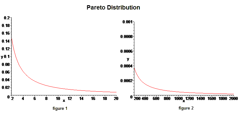
The following picture shows the graph from two sections of the domain of a Pareto distribution where the x-axis is the degree of difficulty of a problem, and the area under the curve between a range of difficulties (for example from 2.4 to 7) is the probability that a random problem is in that range of difficulty.
As you can see in the distribution, most problems are relatively easy to solve. But as can be seen in figure 2 above, the distribution also has a thick “tail” that continues on forever which means that there are many problems that are extremely difficult—many problems with a level of difficulty of every degree.
Given that most problems are relatively simple to solve, it would be a significant waste of time to apply sophisticated and time consuming strategies to solve every problem you face just in case the problem might be a harder problem to solve. Of course due to how common complicated problems exist, there should be strategies to deal with these problems—only after it becomes obvious that the problem is not trivial to solve. In fact, always implementing sophisticated and time consuming strategies when you do not yet know the difficulty of a problem will make solving harder problems even more time consuming. This is because harder problems usually involve several sub-problems, sub-problems of those sub-problems, and so on. If for each of those sub-problems you initially implement a sophisticated and time intensive strategy, then solving your original problem may be so time intensive, that you may never solve your original problem.
It is often hard to know the level of complexity of a problem by first looking at it. So what is needed is a method for problems that are assumed to have little complexity—making the method very fast to implement. If using the fast and simple method doesn't successfully solve a given problem, then it would be necessary to apply methods of problem solving that assume more complexity of the problem. When it becomes obvious that the problem is indeed complex, then it becomes necessary to start the high level time-consuming machinery for problem solving. For example, if you wanted to find your favorite shirt, you wouldn’t start looking by tearing the house apart and looking in every nook and cranny. You would probably start by looking in your closet, or in the laundry room. Then if that strategy failed, you may try a somewhat more sophisticated search, and if that fails, then you might start tearing the house apart looking in every nook and cranny.
Let T be a problem, and C(T) be the complexity of solving problem T—meaning that C(T) is the size of the smallest process (for example a method or algorithm) that solves problem T. (This representation was created by Solomonoff where T was a representation of a theory.) Let W be the set of all finitely written problems T (meaning the problem is written using a finite number of symbols) that are also finitely solvable problems (meaning that the complexity of T is finite). Then C: W → R is a random variable that seems to be Zipf distributed. The Zipf distribution is a discrete form of the Pareto distribution. Given a problem T chosen at random from the problem set W, the utility (or benefits) from solving problem T depends upon the value of solving problem T, and depends on the time it takes to solve problem T. Given a utility function of the time t it takes to solve problem T, U:R+×W→R+, the Intelligence of a problem-solving method with respect to this utility function is defined to be E[U(t(T),T)] which is the expected utility of the time it takes to solve a randomly chosen problem T in W. The overall goal is then to create a general problem-solving method that optimizes this intelligence function. The method that is used to solve problem T is what will then define the function t(T). The method given in the following section is created to try to be as universally intelligent as possible with respect to usual utility functions. Because this method was created by simply using guiding ideas for effective problem-solving, it will not necessarily provide “optimal intelligence”, but is a step in the right direction. More research needs to be done in the field of methods for optimal intelligence.
Steps to Implement the Main Problem-Solving Method
The steps to implement the Main Problem-Solving method are: